


DeepSeek-V3: Understanding and Running the Best Open LLM Locally
A huge but efficient MoE


DeepSeek-V3 is one of the best open LLMs, outperforming most others in various tasks. With 671 billion parameters, you would expect it to require multiple GPU nodes and to run very slowly, even on expensive hardware. However, DeepSeek-V3 is actually much faster than smaller models like Llama 3.3 (70B) and Qwen2.5 (72B).
So, how does DeepSeek-V3 manage to be so efficient despite being so large?
This article will explain how DeepSeek-AI made this possible. They built on their earlier work, DeepSeek and DeepSeek-V2, by using a special mixture of experts model with many smaller expert models, a few shared experts, and multi-head latent attention. They also trained the model to use FP8 precision, making it much more memory-efficient compared to models of similar size.
We’ll also examine the hardware needed to run DeepSeek-V3 and the cost of running a copy of the model in the cloud.
If you want to try it for yourself, my notebook linked below includes vLLM inference code, using multiple GPUs, to get you started with DeepSeek-V3.
DeepSeek-V3: A Huge but Efficient MoE
DeepSeek-AI published a technical report full of details explaining how they trained the model and its architecture:
The main building blocks of DeepSeek-V3, like DeepSeekMoE and Multi-Head Latent Attention (MLA), were first introduced in DeepSeek-V2. They’re built to keep inference fast and memory-efficient despite the huge number of parameters.
What I really love about this architecture is how it packs in so many fresh ideas from state-of-the-art research, along with some really clever engineering tricks. It’s a smart and practical design that just works, and it is all well summarized by this illustration:
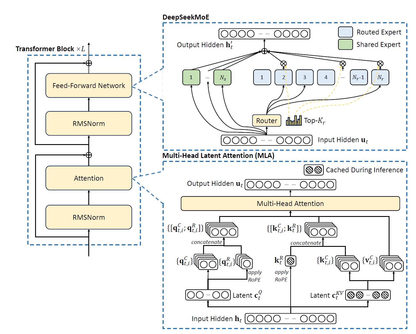
Understanding Multi-Head Latent Attention
Multi-Head Latent Attention is an optimized attention mechanism. It improves memory efficiency while maintaining performance comparable to standard Multi-Head Attention (MHA). One of its main advantages is that it significantly reduces memory consumption during inference, which is caused by the need to store all key-value pairs for each token in the sequence.

The core idea of MLA is to compress the input embeddings into a lower-dimensional latent space before generating the keys and values. Note: Technically, this is not a quantization of the KV cache.
For each token, the embedding is first projected into this compressed latent space using a down-projection operation. From this compressed representation, the keys and values are reconstructed for the multiple attention heads using an up-projection operation. The keys also incorporate positional information through a separate projection that applies Rotary Positional Embedding (RoPE). The final keys used in attention are a combination of the reconstructed keys and the keys carrying positional information. This approach allows the model to store only the compressed latent representations and the positional keys, i.e., reducing the memory required for caching.
Similarly, the queries used in the attention mechanism are also compressed into the latent space, reducing memory usage during training by limiting the size of activations (i.e., the tensors created during inference) that need to be stored. The queries are later reconstructed from the compressed representations for use in the attention computation.
Once the compressed queries, keys, and values are computed and reconstructed, they are used to calculate attention outputs. The queries and keys are used to compute attention weights, which are then applied to the values to produce the output for each attention head. These outputs are concatenated and projected to produce the final attention output for the token.
MLA achieves significant memory savings because only the compressed latent representations for the keys and values, along with the positional keys, are stored during inference.
This is a major improvement over standard MHA, where all keys and values for every token must be cached. Despite these optimizations, MLA retains performance comparable to standard attention mechanisms by accurately reconstructing the necessary information from the compressed representations. This makes it particularly well-suited for applications requiring long sequences or efficient inference.

Shared and Tiny Experts with DeepSeekMoE
In DeepSeek models, Feed-Forward Networks (FFNs) leverage the advanced DeepSeekMoE architecture, originally introduced in DeepSeek (V1). This architecture refines expert segmentation to achieve finer granularity for better specialization and more efficient knowledge acquisition. It also incorporates shared experts to minimize redundancy across routed experts. According to DeepSeek-AI, this architecture improves both knowledge distribution and expert utilization. This seems to be corroborated by their results.
DeepSeekMoE represents a substantial improvement over the conventional Mixture of Experts (MoE) architectures but, as far as I know, DeepSeekMoE hasn’t been used in any other models since they introduced it. Note: If you don’t know how MoE works, I recommend reading my introduction to Mixtral.
To address the communication costs associated with MoE, particularly in multi-GPU hardware configurations, DeepSeek employs a device-limited routing mechanism. In scenarios where expert parallelism is used, routed experts are distributed across multiple devices, with the communication cost for each token depending on the number of devices that its target experts span. This ensures more efficient cross-device communication during inference and training. This is key in the inference efficiency of DeepSeek models as they are designed, due to their size, to be run in multi-GPU settings.
Unlike the simple top-K selection used in traditional MoE architectures, DeepSeek’s routing mechanism enforces an additional constraint: each token's target experts are limited to being distributed across no more than M devices. The process first identifies the top M devices with experts having the highest affinity scores for the token. Within these devices, the top-K selection is then performed to finalize the expert assignments. This approach significantly reduces the communication overhead while maintaining high performance.
To further enhance efficiency, DeepSeek integrates auxiliary losses to manage load balance and prevent routing collapse, a situation where certain experts are underutilized, leading to computational inefficiency. Three types of auxiliary losses have been implemented to achieve this:
Expert-Level Balance Loss is used for equitable token distribution across experts by calculating token-to-expert affinity and applying a balance factor that promotes even load distribution.
Device-Level Balance Loss balances computational loads across devices by organizing experts into groups and spreading them across different devices, ensuring that no single device becomes a bottleneck.
Communication Balance Loss addresses imbalances in inbound communication by equalizing the number of tokens processed by each device, thereby minimizing communication delays.
Then, to address load imbalance, DeepSeek introduces a device-level token-dropping strategy during training. This method computes the computational budget for each device and discards tokens with the lowest affinity scores until the budget is met. To maintain alignment between training and inference, approximately 10% of training sequences are exempt from token dropping. This strategy provides flexibility by enabling token dropping during inference when efficiency is prioritized while preserving high performance in scenarios where full token processing is required.
Multi-Token Prediction
Multi-Token Prediction (MTP) in DeepSeek-V3 is a training objective inspired by previous work, predicting multiple future tokens simultaneously, rather than focusing on one token at a time. This approach densifies the training signals and improves data efficiency by allowing the model to process and learn from multiple future token predictions in a single forward pass.
The MTP mechanism predicts additional future tokens sequentially rather than in parallel. Unlike earlier approaches, which used independent output heads to predict multiple tokens at once, DeepSeek-V3 maintains a complete causal chain during each prediction depth. Each additional token prediction depends on the tokens and predictions from previous steps to preserve the causal structure of the output.
The implementation of MTP involves a series of modules, each designed to predict one additional token at a specific depth. Each module includes a shared embedding layer, a shared output head, a depth-specific Transformer block, and a projection matrix. At each depth, the representation of the current token from the previous depth is combined with the embedding of the next token in the sequence. These representations are concatenated and projected into a new representation that serves as input to the Transformer block for that depth. The Transformer block then processes this input to produce the output representation for the current depth. This output is used by the shared output head to calculate the probability distribution for the predicted token at this depth.

The MTP training objective uses cross-entropy loss to evaluate the predictions at each depth. For each depth, the model compares the predicted probabilities of the next token with the ground-truth tokens in the sequence and computes a loss value. The total MTP loss is then calculated as the weighted average of the losses across all prediction depths, with a weighting factor applied. This loss serves as an additional objective during training, complementing the primary training objectives of the main model.
During inference, the MTP modules are not required for normal functioning and can be discarded. However, the MTP modules can also be repurposed for speculative decoding to improve generation speed by leveraging predictions from earlier depths to precompute subsequent steps.
GPU Requirements for DeepSeek V3
According to DeepSeek-AI, the model has 671B parameters. However, the model card in Hugging Face tells us that the model is slightly larger with 685B parameters:

It doesn’t make a huge difference. The model requires a huge amount of memory anyway. However, since the model natively supports FP8, it means that 1B parameters only cost 1 GB. So we need, 671 GB to load the model, e.g., 4 AMD MI300X, 9 H100 GPUs, or 5 H200 (143 GB each on RunPod).
Recent GPUs, like the H100 and H200, are optimized for fast FP8 processing.
Once the model is loaded, we need additional memory for inference.
To be able to run the model efficiently, possible configurations are:
6 MI300X: the most affordable but relies on AMD software, so it might not work well with some frameworks.
Between 12 and 16 H100s: This is a good alternative but requires more than one GPU node in most configurations (I’m not aware of a machine hosting more than 8 H100s, but it might be possible, let me know in the comments). Multiple nodes tend to increase inference time due to the need for the machines to synchronize with each other.
8 H200s: This is the most expensive but also the fastest and most practical. One node of 8 H200s is enough to run the model.
I would opt for the configuration with 8 H200s. On RunPod (referral link), you can get one for $32/hour (as of January 3rd, 2025), plus a few dollars for storage. Unfortunately, this configuration is still rarely available.
Running DeepSeek-V3 Locally, Is It Possible?
For the FP8 version
Yes, it’s possible but you need a GPU node. Given that a single node with 8 H200 GPUs is currently priced at $260k (when it's even available), the cloud proves to be a much more cost-effective option. For example, using RunPod's current pricing as a baseline, you’d have to run your node continuously for over a year before you’d begin saving money compared to leveraging cloud services.
SGLang and vLLM both support FP8 models.
I have less experience with SGLang (but it’s a good framework). With vLLM, we must pass the following arguments to the engine for distributed inference:
tensor_parallel_size = 8 (if you have 8 GPUs)
pipeline_parallel_size = 2 (if you have two nodes)
You can run the model with this engine configuration if you have enough memory in a single node, e.g., using 8 H200s:
llm = LLM(model="deepseek-ai/DeepSeek-V3", tensor_parallel_size=8)If you have several GPU nodes, e.g., 2 nodes of 8 H100s each, you can do pipeline parallelism in addition to tensor parallelism:
llm = LLM(model="deepseek-ai/DeepSeek-V3", tensor_parallel_size=8, pipeline_parallel_size=2)For the INT4 version, quantized with AutoRound
The Open Platform for Enterprise AI (OPEA) has released a 4-bit version of the model made with AutoRound, formatted in GPTQ so you can use it with vLLM. The model was quantized by the creators of AutoRound. Note: Interestingly, it seems they opted to release it under OPEA instead of Intel, possibly to sidestep Intel’s bureaucratic hurdles for approving new model releases. (my guess)
OPEA/DeepSeek-V3-int4-sym-inc-cpu (MIT license)
The model can run on a single node of 8 H100s.
OPEA couldn’t run an evaluation of the model due to a lack of funding (according to the model card; this doesn’t make sense to me since the quantization itself costs much more than the evaluation). I estimate that evaluation would cost a few hundred dollars with standard non-generative benchmarks (e.g., MMLU, GPQA, and MuSR).
Given the model's large size and the fact that 4-bit quantization is typically highly accurate for large models, this 4-bit version is likely to perform on par with the original. However, this assumption should be thoroughly validated, as some layers may not be properly quantized with AutoRound, which could result in the model generating nonsensical outputs.
I also assume that a 2-bit version could be extremely accurate. Hopefully, OPEA will release one.
Conclusion
If we look at the benchmark results, DeepSeek-V3 is the best open LLM (MIT license for the code; DeepSeek license for the model).

While using it for daily tasks is currently impractical—or at least not cost-effective—I anticipate the release of smaller, more efficient models in the coming months, likely trained using DeepSeek-V3 through the teacher-student framework, also known as knowledge distillation.
I haven’t even mentioned it yet, but the most impressive part of this work is, in my opinion, the extreme optimization of the training. A pre-training of a 671B parameter model with a standard training pipeline is extremely expensive (much more than $10 million).
DeepSeek-AI provides many details on how they extremely optimized their training pipeline to perfectly match their hardware configurations. The training of DeepSeek-V3 is highly economical. Pre-training on one trillion tokens required 180,000 H800 GPU hours, equivalent to 3.7 days using a cluster of 2,048 H800 GPUs. The full pre-training stage was completed in under two months, using 2,664,000 GPU hours. Including 119,000 GPU hours for context length extension and 5,000 GPU hours for post-training, the total training time amounts to 2.788 million GPU hours. At a rental rate of $2 per GPU hour, the total training cost is $5.576 million. Impressive!
DeepSeek on a budget!